Eigenvalue Calculator: Exact Eigenvalues, Eigenvectors and Steps
Exact eigenvalues the way a grader writes them, as fractions, √ surds and a ± bi, come out of this eigenvalue calculator next to the decimals, each with its eigenvector. Enter any matrix from 2×2 to 6×6 to see the characteristic polynomial, the multiplicities, whether A = PDP⁻¹ exists, and the hand steps.
Enter a square matrix from 2×2 up to 6×6, typed cell by cell or pasted as text, and the eigenvalue calculator above returns the eigenvalues with their multiplicities, an eigenvector for every one of them (complex ones included), the characteristic polynomial, the trace and the determinant. When every entry is an integer, a fraction such as 1/2 or a terminating decimal, the work is done in exact arithmetic, so you see (1 ± √5)/2 or 2 ± i the way a grader writes it, with the decimal beside it. It also says whether A = PDP⁻¹ exists (over the real numbers, only over the complex numbers, or not at all because the matrix is defective), writes out the hand steps at every size, draws what a 2×2 matrix does to the plane, and checks every eigenpair against Av = λv before you copy the result. Entries may be typed with a decimal point or a decimal comma, and the result can be copied as LaTeX, plain text, NumPy code or a share link.
Eigenvalues of a 2×2 matrix by hand
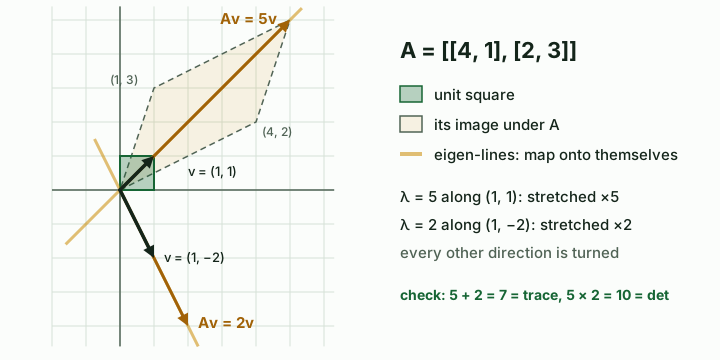
Take A = [[4, 1], [2, 3]]. Subtract λ from the diagonal and set the determinant to zero:
So λ = 5 and λ = 2. Once students have done the long way a few times, I let them use the 2×2 shortcut. With trace tr = 4 + 3 = 7 and determinant det = 4·3 − 1·2 = 10:
That gives 5 and 2 again. Eigenvectors come from the null space of A − λI, one eigenvalue at a time:
- λ = 5: A − 5I = [[−1, 1], [2, −2]]. Both rows say −x + y = 0, so y = x and v = (1, 1).
- λ = 2: A − 2I = [[2, 1], [2, 1]]. One equation, 2x + y = 0, so y = −2x and v = (1, −2).
- Check: 5 + 2 = 7 is the trace, 5 · 2 = 10 is the determinant, and A(1, 1) = (5, 5) = 5·(1, 1).
If A − λI keeps full rank (no row becomes a multiple of the other), your λ is wrong; go back to the polynomial before you hunt for a vector. The shortcut also tells you what kind of answer to expect: tr²/4 − det positive means two real eigenvalues, zero means one repeated eigenvalue, negative means a complex conjugate pair.
A 3×3 example: expand along the row with zeros
For A = [[2, 0, 0], [1, 2, −1], [1, 3, −2]] I expand det(A − λI) along the first row, because two of its entries are zero:
The roots are λ = 2, 1 and −1. The calculator prints the monic form p(λ) = det(λI − A) = λ³ − 2λ² − λ + 2. For a 3×3 (odd n), det(A − λI) = −det(λI − A); the roots are the same, so a polynomial with every sign flipped against the answer key is not a mistake.
| λ | A − λI | RREF reads | Eigenvector |
|---|---|---|---|
| 2 | [[0, 0, 0], [1, 0, −1], [1, 3, −4]] | x = z, y = z | (1, 1, 1) |
| 1 | [[1, 0, 0], [1, 1, −1], [1, 3, −3]] | x = 0, y = z | (0, 1, 1) |
| −1 | [[3, 0, 0], [1, 3, −1], [1, 3, −1]] | x = 0, z = 3y | (0, 1, 3) |
Check: 2 + 1 + (−1) = 2 = trace, and 2 · 1 · (−1) = −2 = det A. Without a convenient zero row, use the rational-root test on the monic polynomial: for an integer matrix every rational eigenvalue is an integer that divides the constant term. When none of the candidates works, as with [[4, 2, 1], [2, 5, 3], [1, 3, 6]] and p = λ³ − 15λ² + 60λ − 67 (candidates ±1 and ±67), the roots are irrational, ≈ 9.348494, 3.730159 and 1.921347, and a numerical answer is the honest one. The full hand method, synthetic division included, is in how to find eigenvalues and eigenvectors.
Why your eigenvectors differ from NumPy’s
An eigenvector is a direction, not a fixed list of numbers: any nonzero multiple of v is also an eigenvector. Textbooks scale to the smallest integers, and so does this eigenvalue calculator, so for λ = 5 above you see (1, 1). numpy.linalg.eig and MATLAB’s eig return unit-length columns, so the same direction prints as (0.7071, 0.7071). For λ = 2 NumPy gives (−0.4472, 0.8944): that is (1, −2) divided by √5 and multiplied by −1. Divide every entry by the first nonzero one and both answers become (1, −2). That single division settles nearly every “the software disagrees with me” question.
Repeated eigenvalues: count the free variables
Repeated roots are where most diagonalization marks are lost. The number of times λ repeats as a root is its algebraic multiplicity. The number of free variables in the RREF of A − λI, that is n minus its rank, is its geometric multiplicity: the dimension of the eigenspace. A matrix is diagonalizable exactly when the two numbers agree for every eigenvalue.
| Matrix | λ | Algebraic | Geometric | Verdict |
|---|---|---|---|---|
| [[2, 1, 1], [1, 2, 1], [1, 1, 2]] | 4 1 | 1 2 | 1 2 | diagonalizable; eigenspace of 1 spanned by (−1, 1, 0) and (−1, 0, 1) |
| [[3, 1], [0, 3]] | 3 | 2 | 1 | defective; only (1, 0) |
| [[0, 1, 0], [0, 0, 1], [8, −12, 6]] | 2 | 3 | 1 | defective; only (1, 2, 4) |
The first matrix is symmetric, and a real symmetric matrix is always diagonalizable, with real eigenvalues and orthogonal eigenvectors (the spectral theorem), however many repeats it has. For the other two no choice of P works; the nearest thing is the Jordan form. Distinct eigenvalues always give a diagonalization, so free variables only need counting at the repeated ones. Worked cases, generalized eigenvectors included, are in repeated eigenvalues and diagonalization.
Complex eigenvalues are still eigenvalues
A = [[1, −2], [1, 3]] has trace 4 and determinant 5, so tr²/4 − det = 4 − 5 = −1 and λ = 2 ± i. “No real eigenvalues” does not mean “no eigenvalues”. The eigenvector comes from the first row of A − (2 + i)I = [[−1 − i, −2], [1, 1 − i]]: (−1 − i)x − 2y = 0, so x = 2, y = −1 − i and v = (2, −1 − i). For a real matrix the partner comes free: conjugate everything, λ = 2 − i with v = (2, −1 + i).
Read the pair as scaling plus rotation, up to a change of basis. The modulus |λ| = √5 ≈ 2.236 is the stretch per step and the argument, about 26.57°, is the turn per step, so repeated multiplication by A spirals outward. With |λ| below 1 the spiral goes inward; at exactly 1 it is a pure rotation, as with [[0, −1], [1, 0]], whose eigenvalues are ±i. The guide to complex eigenvalues and eigenvectors takes this further.
What eigenvalues tell you in a model
- Markov chain. The column-stochastic matrix [[0.9, 0.5], [0.1, 0.5]] has λ = 1 and λ = 0.4. The eigenvector for 1 is (5, 1); scaled to sum 1 it is the steady-state vector (5/6, 1/6), about 83.3 % and 16.7 %. The second eigenvalue sets the pace: the gap to the steady state shrinks by a factor of 0.4 every step.
- Leslie population matrix. [[0, 1.5, 0.4], [0.6, 0, 0], [0, 0.8, 0]] has the dominant eigenvalue λ ≈ 1.041335, so in the long run the population grows about 4.13 % per time step. Its eigenvector, scaled to sum 1, is the stable age structure: ≈ 49.5 %, 28.5 % and 21.9 %.
- Fibonacci numbers. [[1, 1], [1, 0]] gives λ² − λ − 1 = 0, so λ = (1 ± √5)/2 ≈ 1.618034 and −0.618034; the golden ratio is the growth rate of the sequence.
- Matrix powers. With A = PDP⁻¹, A⁵ = PD⁵P⁻¹. For A = [[4, 1], [2, 3]], P = [[1, 1], [1, −2]] and D⁵ = diag(3125, 32), and the product is [[2094, 1031], [2062, 1063]] without four matrix multiplications.
Checks I run before trusting any eigenvalue calculator
- Sum of the eigenvalues = trace, product = determinant. It takes a minute and catches most arithmetic slips.
- Triangular matrix: the eigenvalues are the diagonal entries; there is nothing to compute.
- Never row-reduce A before looking for eigenvalues. Row operations change them. Row-reduce A − λI, after λ is known.
- λ = 0 is an eigenvalue exactly when det A = 0: the matrix is singular, and its eigenvectors for 0 form the null space of A.
- A real symmetric matrix has only real eigenvalues. A complex result there means a typo in the entries.
- The eigenvalues of A + B are not the sums of the eigenvalues of A and B; compute them fresh.
- Plug back in: Av must equal λv entry by entry.
Most of these rules are in section 6.1 of Strang’s Introduction to Linear Algebra, still the clearest first reading on eigenvalues I know.
Exact arithmetic first, floating point second
For integer, fraction and terminating-decimal input, at every size from 2×2 to 6×6, the calculator builds the characteristic polynomial in exact rational arithmetic (the Faddeev–LeVerrier recursion on big-integer fractions) and splits off repeated factors. It pulls out rational roots with the full p/q rational-root test; when the constant term is too large to list its divisors, numeric roots are rounded to candidates and each candidate is checked exactly. A leftover quadratic factor is solved exactly as a surd, written like 1 + √2/2 or (1 + √5)/2, or as a ± bi. Rational eigenvalues get exact eigenvectors from the rational RREF of A − λI, scaled to integers with gcd 1. A factor with no exact form is solved numerically and marked with “≈”. That numerical engine is the standard one: balancing, reduction to Hessenberg form, then the QR algorithm with Francis double shifts and exceptional shifts, which handles complex pairs in real arithmetic and does not stall on rotations and permutations; symmetric matrices go through Jacobi rotations instead. When the entries are too large for exact arithmetic the whole answer is numerical, and the page says so. Tolerances are relative to the size of the matrix, so entries near 10⁸ are treated like entries near 1, and an iteration that fails to converge produces an error message, never a guess.
Exact mode matters most for repeated roots, because floating point cannot separate them cleanly: NumPy returns the triple eigenvalue 2 of [[0, 1, 0], [0, 0, 1], [8, −12, 6]] as 2.000019 and 1.999991 ± 0.000016i. Defective matrices are badly conditioned, symmetric ones are well conditioned (see the eigenvalue algorithm and QR algorithm overviews). There is no root formula for polynomials of degree five and up (Abel–Ruffini), so large matrices are always solved iteratively. Every answer carries its own proof: the relative residual ‖Av − λv‖ / (‖A‖·‖v‖) for each eigenpair, which must be below 10⁻⁹ to earn a ✓, and Σλ against the trace and Πλ against the determinant. Some of the control cases the tool is tested against:
| Matrix | Expected eigenvalues | Eigenvectors | Verdict |
|---|---|---|---|
| [[4, 1], [2, 3]] | 5, 2 | (1, 1), (1, −2) | diagonalizable over ℝ |
| [[1, −2], [1, 3]] | 2 ± i | (2, −1 − i), (2, −1 + i) | diagonalizable over ℂ only |
| [[0, 1, 0], [0, 0, 1], [8, −12, 6]] | 2 (algebraic 3, geometric 1) | (1, 2, 4) | defective |
| [[0, 0, 1], [1, 0, 0], [0, 1, 0]] | 1, −1/2 ± (√3/2)i | (1, 1, 1) for λ = 1 | diagonalizable over ℂ only |
| [[1/2, 1/4], [1, 3/2]] | 1 ± √2/2 (≈ 1.7071 and 0.2929) | exact surds, with the last entry of each vector equal to 1 | diagonalizable over ℝ |
| [[0.9, 0.5], [0.1, 0.5]] | 1, 2/5 | (5, 1); steady state (5/6, 1/6) | diagonalizable over ℝ |
| [[1e8, 1], [1, 1e8]] | 100000001, 99999999 | (1, 1), (1, −1) | diagonalizable over ℝ |
| the 6×6 Example preset | 6, 4, 3, 1, −1, −2 | found exactly | diagonalizable over ℝ |
Guides
- How to Find Eigenvalues and Eigenvectors by Hand: 2×2 and 3×3The full hand method for 2×2 and 3×3 matrices, with two worked examples, an irrational cubic and the trace and determinant checks.Reading time: 7 min
- Repeated Eigenvalues and Diagonalization: When A = PDP⁻¹ FailsAlgebraic versus geometric multiplicity, a diagonalizable example, two defective ones, the Jordan chain and A⁵ computed with PDP⁻¹.Reading time: 8 min
- Complex Eigenvalues and Eigenvectors: What a ± bi Tells YouComplex eigenvalues a ± bi: a worked 2×2, the complex eigenvector, modulus and angle, the real rotation-scaling form and a 3×3 permutation.Reading time: 7 min
FAQ
What does a zero eigenvalue mean?
The matrix is singular: det A = 0, it has no inverse, and Ax = 0 has nonzero solutions. The eigenvectors for λ = 0 are exactly the null space of A.
Is the sum of the eigenvalues always equal to the trace?
Yes, as long as you count every eigenvalue with its algebraic multiplicity and include complex ones. The product of the eigenvalues, counted the same way, equals the determinant.
Can a real 3×3 matrix have only one real eigenvalue?
Yes. The cyclic permutation [[0, 0, 1], [1, 0, 0], [0, 1, 0]] has λ = 1 and the complex pair −1/2 ± (√3/2)i. A real 3×3 always has at least one real eigenvalue, because complex ones come in conjugate pairs.
What is the difference between algebraic and geometric multiplicity?
Algebraic multiplicity is how many times λ is a root of the characteristic polynomial; geometric multiplicity is how many independent eigenvectors it has, n minus the rank of A − λI. When the geometric one is smaller for some λ, the matrix is defective and not diagonalizable.
Why is there no formula for the eigenvalues of a 5×5 matrix?
The characteristic polynomial has degree 5, and by the Abel–Ruffini theorem there is no general root formula in radicals from degree five on. Calculators and libraries find these eigenvalues iteratively, with the QR algorithm.
How do I find the steady state of a Markov chain with eigenvectors?
For a column-stochastic matrix (columns sum to 1), take the eigenvector for λ = 1 and divide it by the sum of its entries. If your rows sum to 1 instead, use the transpose of the matrix.